

 LinkedIn

How-it-works ads came in 18% below their account’s average cost per result in the median account. That is a reason to investigate the format, not a forecast of what happens when you give it more budget.
The distinction gets lost somewhere between the analysis and the slide that says “scale the winners.” A cheaper ad becomes a budget recommendation without anyone measuring what the extra results will cost.
I used to make that mistake myself. I would find a creative with a clean cost per result, move money to it on a Friday, then watch the CPA climb back toward average by Wednesday. Blaming the algorithm was easier than admitting I had answered the wrong question.
Biddyco’s published analysis gives us a useful way to separate those questions. It shows which creatives performed efficiently inside spend that already happened. It does not establish how much efficient spend those creatives can absorb next.
What the creative figures actually measure
Biddyco examined 483 top-spending creatives across 17 large US Meta accounts, representing $5.1 million in spend from August 28 to September 26, 2026. That was about two-thirds of those accounts’ spend during the period.
The method matters: compare each creative tag’s cost per result with its own account average, then take the median across accounts. That keeps one enormous spender from dominating the headline.
| Creative category | Median difference from its own account’s average cost per result |
|---|---|
| How-it-works | 18% below |
| Features and benefits | 14% below |
| Polished creative | 4% below |
| Creator-led | 10% above |
These are relative costs among creatives that already received substantial spend. They are useful evidence about the selected ads, not a promise about the next budget increase.
Before using any of those gaps, I want to know what sits underneath “result.”
“Cost per result” is not a common currency
Meta’s cost per result is spend divided by results. The result depends on the campaign’s objective, settings, and attribution window. A purchase and a landing page view can both occupy that column. They are not interchangeable outcomes.
I have been fooled by the tidy version of this report: sort by cost per result, admire the cheapest row, then discover it was optimizing for ThruPlay while the others were optimizing for purchases. The spreadsheet was correct. My interpretation was not.
Roaz states the comparison rule plainly: compare cost per result only when the result type and attribution setting match. Otherwise, use an explicit measure such as cost per purchase or cost per lead.
Biddyco’s account-relative approach avoids pooling raw costs from different businesses. But normalizing against an account average does not, by itself, make every underlying result comparable. The meaning of the baseline still matters, especially if it blends objectives or attribution settings.
I read “below account average” as the beginning of an investigation. I still need to know what the ad and its comparator were trying to achieve.
Follow the denominator from accounts to eligible purchases
A separate Biddyco analysis compares static and video ads. Keep this dataset separate from the creative-tag figures above; its selection and reporting period differ.
It starts with 17 US accounts spending at least $100,000 each over June–August 2026. Biddyco selected the highest-spending ads from each account, producing a pool of ads that had already attracted budget.
That is the first limit: this is not a record of every creative launched, including every abandoned test.
The performance comparisons narrow the pool again. Ads needed at least $1,000 in spend, and purchase comparisons required enough purchases from both formats within an account.
| Selection step | What remains | What the figure can tell us |
|---|---|---|
| 17 accounts; top 50 ads per account | 848 ads and $14.9 million in combined spend | What attracted spend in these large accounts, not every test or small-account experience |
| Format split within that pool | 340 statics and 508 videos; statics represent 40% of ads and 32% of spend | Statics have a substantial presence among selected ads |
| Highest-spending tier | 170 top-10 ads: 73 statics and 97 videos | Statics remain represented among the biggest spend recipients |
| Purchase-comparison subset | 12 accounts with at least 20 purchases per format | A narrower comparison of observed purchase efficiency |
Within that last subset, statics were within 4% of video on cost per purchase in the median account and won in 8 of 12 accounts.
The purchase denominator is the eligible subset, not the whole account pool. Accounts with thin purchase data are already outside the frame. That is a disclosed limit, not a flaw to conceal. The problem starts when someone turns the result into a claim about every advertiser.
Spend share does not tell us sales share
In the static-versus-video analysis, video received 68% of spend and statics received 32%; the median account allocated 37% to statics.
Those figures describe where the money went. They do not say statics generated the same share of purchases, or that assigning the same budget split elsewhere reproduces the result.
Media buyers and Meta’s delivery system put money behind promising signals. The ads that survive receive more. By the time we examine the highest-spending group, selection has already done plenty of work.
The efficiency figures add useful detail: statics had 15% lower CPM and 13% lower link CTR in the median account, while purchase costs in the eligible subset remained close to video’s. Cheaper impressions and fewer clicks did not automatically translate into worse purchase economics.
That challenges video-only dogma. It does not establish a static budget quota.
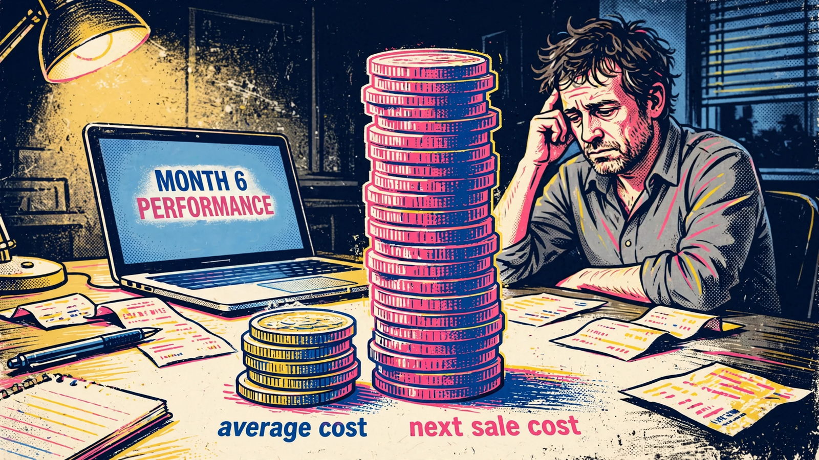
Spend share measures allocation; cost per purchase measures observed efficiency. Neither measures the price of expanding delivery. For that, I need marginal cost.
The next purchase can cost more than the dashboard average
Marginal CPA is extra spend divided by extra purchases. It asks a different question from average CPA: what did the increase buy?
The arithmetic is easier to see than the jargon.
| Illustrative daily result | Before the increase | After the increase |
|---|---|---|
| Spend | $100 | $200 |
| Purchases | 5 | 8 |
| Average CPA | $20 | $25 |
The additional $100 buys 3 additional purchases, or roughly $33 each. With an illustrative breakeven CPA of $30, the extra spend loses money even though the blended average remains below breakeven.
This is an illustration, not a result from Biddyco’s accounts. Nor does a before-and-after calculation, on its own, prove that the budget change caused every difference. It makes the economic question visible.
A winning creative’s historical average includes the delivery it has already received. More budget may require reaching less responsive people or buying less efficient inventory. The earlier average does not price that expansion.
I want to price the next lead, not admire the average. That is the number a scaling decision needs.
A cheap workhorse is not proof of cheap scale
A companion analysis reinforces the distinction. In a wider pull of 34 accounts, 23 had static and video options with enough spend to compare; a static was the cheapest workhorse in 12 of those 23.
Useful evidence against dismissing statics. Still not a scaling plan.
The comparator does quiet work here. An account average can blend prospecting and retargeting, cheap remarketing and expensive cold reach, or campaigns pursuing different outcomes. Beating that blend is not the same as beating a matched alternative at the same budget.
I used to tell clients the winner would hold. I was wrong to make that a promise. What matters is whether the conditions that made it cheap survive the increase.
The usual post-scale failure modes give me a practical list to investigate:
- Delivery reaches less responsive people after the easiest conversions.
- Budget changes bring renewed learning and volatility.
- Frequency rises while click-through rate fades.
- Extra spend reaches weaker ads that previously received little budget.
- Duplicated campaigns compete rather than solve the underlying problem.
A plausible failure mechanism is a monitoring plan, not evidence that failure is inevitable. Before increasing spend, I want the manager to name what they will watch and what would make them reverse the decision.
What these datasets leave unanswered
The published figures stop short of the questions that determine whether a business should spend more. I keep those gaps separate rather than filling them with confidence.
- Marginal cost. We have averages among selected ads, not a measured cost curve showing what happens as each winner receives more budget.
- Downstream quality. A cheap lead that never answers the phone can be worse value than a more expensive lead that books. Cost per result does not settle that.
- Profit. Without contribution margin and breakeven CPA, a relative efficiency gap does not establish an acceptable acquisition cost.
- Stability at higher spend. A snapshot of ads that received budget is not a test of what happens when a particular tag receives substantially more.
Medians also leave an important question open: how widely do outcomes vary? They keep a large spender from dominating the summary, but the median alone cannot show how often the apparent advantage reverses or how much purchase data supports each account’s result.
An outside benchmark cannot supply that missing distribution. Triple Whale’s benchmark covers more than 40,000 brands from August 2025 to July 2026, reporting median CPA of $38.99, CPM of $15.06, conversion rate of 1.53%, and ROAS of 1.88.
That tells me something about the water level in the harbor. It does not tell me whether my boat leaks.
A network benchmark cannot answer an account-specific marginal-cost question. If a manager cites it to justify more budget, they are answering a different question.
What I require before approving more budget
Before I let anyone scale a winner, I ask for a short written case. Not a victory lap around the cheapest row.
- Define the baseline. State the comparison dates, the account average, and exactly what counts as a result.
- Match the outcome. Use the same event and attribution window. For lead generation, put lead quality and close rate beside acquisition cost. Creative cost is only one input into what a lead ultimately costs.
- Show the spend range. Identify where the apparent efficiency held and what happened during the last increase. Separate the marginal calculation from the blended average.
- Set the reversal rule. Agree on the marginal CPA that makes us pause or move budget back, with downstream quality included in the decision.
If those answers are missing, the budget slider stays where it is.
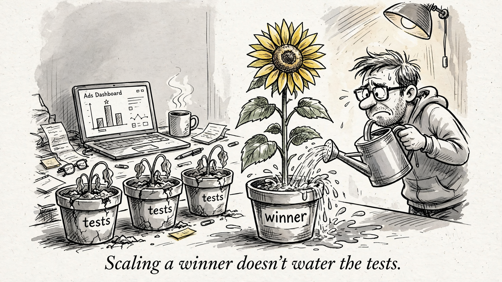
The next step is a limited increase with the comparison defined in advance: track extra spend, extra purchases or qualified leads, and whether sales accepts those leads. Watch frequency, click-through rate, and where the additional budget actually goes. Treat the resulting marginal calculation as evidence to assess, not automatic proof of causation.
If the extra results remain below breakeven and retain their quality, there is a case for another increase. If they do not, a flattering historical average is no reason to continue.
A cheaper ad is worth investigating. Scale only when the marginal economics support it.


